by R. Grothmann
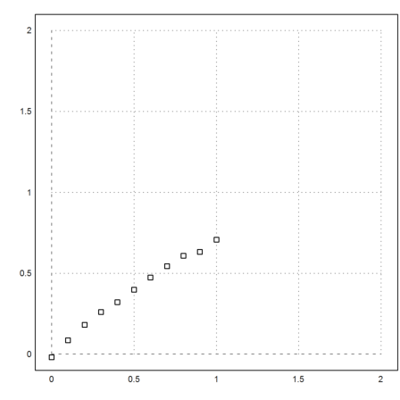
In this notebook, we want to test a linear regression with quadratic polynomials. First let us generate a random scatter of the polynomial 0.1x^2+0.9x^2 at 11 points, evenly spaced in [0,1].
>seed(0.5); a=-0.2; b=0.9; ...
   x:=0:0.1:1; y:=a*x^2+b*x+0.01*normal(size(x)); ...
   plot2d(x,y,a=0,b=2,c=0,d=2,points=1):
It is easy to find the best fit, i.e., the polynomia p of degree 2, which minimizes
![]()
>p:=polyfit(x,y,2)
[-0.0110893, 0.956947, -0.246374]
We add this to our plot.
>plot2d("evalpoly(x,p)",add=1):
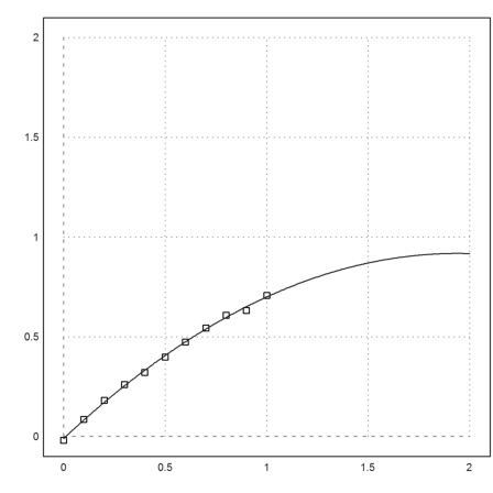
We have used the measurements to extrapolate the data in [1,2].
How can we check the error of this procedure?
Here is one method, which does not work: We assume, that we could just as well have got any data between our measurements, and the values of our estimated polynomial. This is reasonable. We extrapolate from any of these hypothetical data with a polynomial fit. Where would we get?
A simple interval analysis fails by overestimating the error grossly.
>yp:=evalpoly(x,p); yi:=~y~||~yp~;
yi are the intervals betwee y (measurements) and yp (estimated true values). We solve the normal equation of polynomial fit in an interval fashion.
>A:=(1_x_x^2)'; bi:=ilgs(A'.A,A'.yi')
                              ~-0.13,0.1~
                           ~0.3223,1.592~
                             ~-0.84,0.35~
This is a very bad result.
So we try a Monte Carlo simulation. 1000 times, we select random y-values between y and yp, and compute the minima and maxima of all extrapolations for t between -0.5 and 1.5.
>function test (t,x,y,yp,n=1000) ...
   yr=yp+random(size(yp))*(y-yp);
   smin=evalpoly(t,polyfit(x,yr,2));
   smax=smin;
   loop 1 to n;
     yr=yp+random(size(yp))*(y-yp);
     s=evalpoly(t,polyfit(x,yr,2));
     smin=min(smin,s);
     smax=max(smax,s);
   end
   return {smin,smax};
 endfunction
Now plot all that in one figure.
>plot2d(x,y,a=0,b=2,c=0,d=2,points=1);
Compute the Monte Carlo simulation.
>t=0:0.05:2; {smin,smax}=test(t,x,y,yp);
Add it to the plot.
>plot2d(t,smin_smax,add=1,color=5):
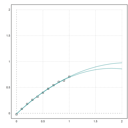
This does not look bad.
But one could argue, that the plot shows that we almost have no information at all. Any schoolboy would give a point in the range, when asked to predict a value for 1.4.
The maximal error is more than 10 times larger than the random error, we started with.
>max(smax-smin)
0.117942934541
Another way to look at this is to simulate 0-0.1-normal distributed scatter of the correct polynomial, and study the distribution of the extrapolation in 2.
>x:=0:0.1:1; yt:=a*x^2+b*x;
We do that 1000 times.
>n:=1000; s=zeros(1,n); ...
 loop 1 to n; s[#]:=evalpoly(2,polyfit(x,yt+0.01*normal(size(x)),2)); end;
The results are randomly distributed around the expected value 3.8. (the value of the exact polynomial at 2).
>plot2d(s,>distribution):
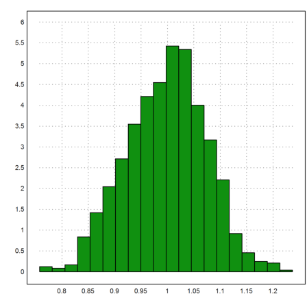
>mean(s), dev(s)
0.998140239383
0.0753540474408
The standard deviation of the extrapolated values is typically much larger than the deviation of the data. It is simply not a good idea to extrapolate thus far with so little information.